NLP Notes

19 minute read

4 Regular Expressions

Square brackets […]: Matches a single character within the brackets
Ranges […-…]: Matches any one of the characters defined in a range
Negations [^…]: Carat means negation when it is the first character after [
Disjunctions : Or
Wildcard: . Matches any character except a carriage return (\r) except newline
- [0-9.] matches either a digit or a period. Inside square brackets a period is a period. Outside square brackets a period is a wild card character
? Optional. Repeats a character 0 or 1 time
* Repeats a character 0 or more times: [abc]* aabbabc
+ Repeats a character 1 or more times

Escaped special characters

. Matches a dot . * Matches an asterisk * + Matches a plus sign + \ Matches a backslash
\n Matches a new line \t Matches a tab \r Matches a carriage return

\r: return to the beginning of the current line without advancing downward

{3} Exactly 3 times
{3,} 3 or more times
{3, 5} Between 3 and 5 times

Anchors

^ Matches the start of a line $ Matches the end of the line

^[A-Z] Ankara … ^[^A-Z] 06 Ankara. ‘‘Ankara’’ .$ The end. The end! The end .$ The end. ^abc$ abc

\s [\t\r\n\f] any whitespace
\S [^\s] any non-whitespace
\d [0-9] any digit
\D [^0-9] any non-digit
\w [a-zA-Z0-9_] any alphanumeric or underscore
\W [^\w] any non-alphanumeric
Paranthesis operators ( and ) Enclosing a pattern in paranthesis makes it act like a single character (the) a (an) the or a or an

Operator Precedence

From highest precendence to lowest in following order:

Paranthesis ( )
Counters * + ? { }
Sequences and anchors the ^ $
Disjunction

Regular expression patterns are greedy. They match the largest string possible. How to enforce non-greedy matching? “+?” “*?” It matches as little as possible

Grep Command: Global Regular Expression Print

5 Text Processing

Sentence segmentation
Tokenization:
- The task of chopping a sentence up into tokens (words or terms)
Token Normalization: Tokens in multiple forms should be normalized into a single form
- Case folding: Lower case all letters
- Stemming: Reducing words to their stems
  - Morphological Analysis for Turkish
  - Porter stemmer: The most common English stemmer, list of rules
  - Krovetz Stemmer: Hybrid algorithmic-dictionary
Stopword removal: Stopwords: Mostly function words
- Determiners (the, a, an)
- Prepositions (in, on, at, …)
- Conjunctions (and, but)

Text Processing Steps: Must be fast, use regex

Sentence segmentation
Tokenization
Token Normalization
- Case folding
- Stemming
Stopword removal

7 Statistical Properties of Text

Zipf’s Law

George Kingsley Zipf

Term frequency decreases rapidly as a function of rank!

ft = k / rt

ft = frequency (number of times term t occurs)
rt = frequency-based rank of term t
k = constant (specific to the collection)

Pt = c / rt

Pt = proportion of the collection corresponding to term t
c = constant
For English c = 0.1 (more or less)

What does this mean?

The most frequent term accounts for 10% of the text • The second most frequent term accounts for 5% • The third most frequent term accounts for about 3% • Together, the top 10 account for about 30% • Together, the top 20 account for about 36% • Together, the top 50 account for about 45%

With some crafty manipulation, it also tells us that the faction of terms that occur n times is given by: 1 / n(n+ 1)

• About half the terms occur only once! • About 75% of the terms occur 3 times or less! • About 83% of the terms occur 5 times or less! • About 90% of the terms occur 10 times or less!

Vocabulary Growth and Heaps’ Law

• The number of new words decreases as the size of the corpus increases • Heaps’ Law: v =k × n(to β) • v = size of the vocabulary (number of unique words) • n = size of the corpus (number of word-occurrences) • k = constant (10 ≤ k ≤ 100) ‣ not the same as k in Zipf’s law • B = constant (B ≈ 0.50)

9 Minimum Edit Distance

The minimum number of editing operations needed to transform one string into another

Insertion
Deletion
Substitution

Used to estimate lexical similarity between to strings

Alignment: A correspondence between substrings of the two sequences.

Levenshtein Distance

Levenshtein distance between two sequences

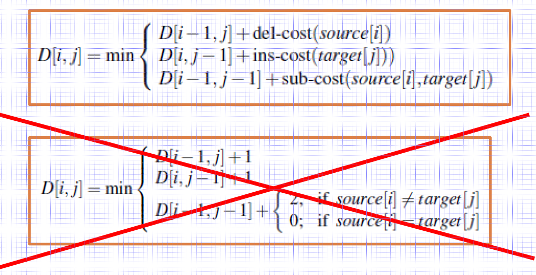
each of the three operations has a cost of 1
the substitution of a letter for itself has zero cost

Convert intention to execution - it has distance of 5 or 8 depending on how to count “s” 1 or 2 operations.

Dynamic Programming

Solving a complex problem by breaking it down into simpler subproblems.
Solving each of those subproblems just once, and storing their solutions.
The next time the same subproblem occurs, instead of recomputing its solution, one simply looks up the previously computed solution.
X: Source string of length n
Y: Target string of length m
D(n,m): The edit distance between X and Y
X[1..i]: the first i characters of X
Y[1..j]: the first j characters of Y
D(i,j): the edit distance between X[1..i] and Y[1..j]

Intention-Execution Min Edit Distance Matrix Calculation

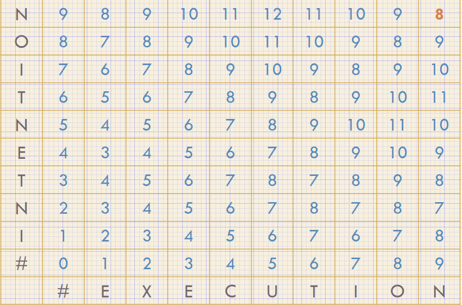
The edit distance is not sufficient

The alignment between the two strings is required
We need to keep additional information
Which operation applied to which character
We need to keep a backtrace

Performance:

Time: O(nm)
- We need to fill nm cells
Space: O(nm)
- Matrix has nm cells
Backtrace: O(n+m)
- In the worst case, n deletions and m insertions

Weighted Edit Distance

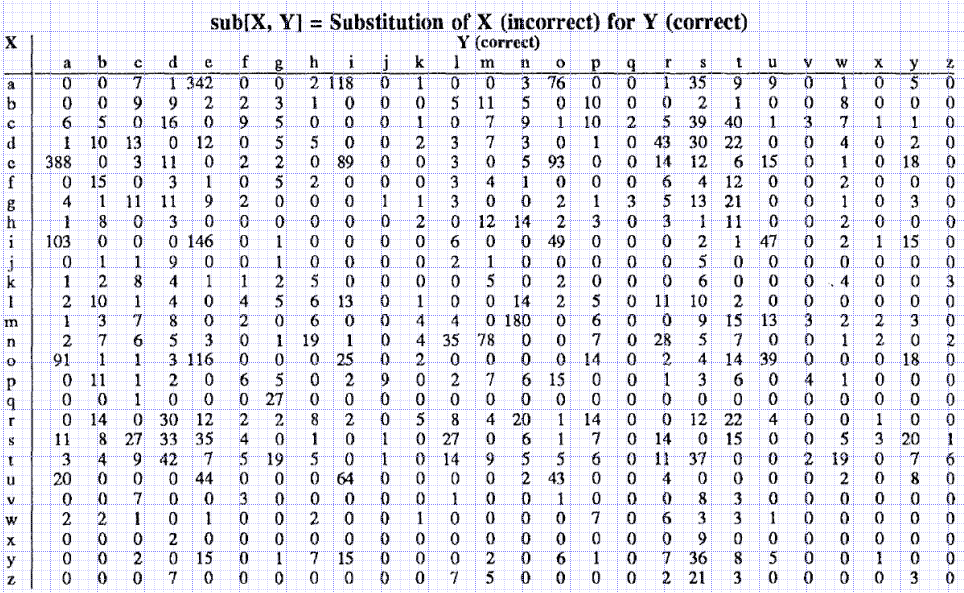
Some letters are more likely to be mistyped than others

Confusion Matrix for Spelling Errors

10 - Language Modeling

One of the hardest topics in NLP (Natural Language Processing) is the Sentiment Analysis topic. It is to decide whether the given document, sentence, aspect, or word is positive, neutral or negative in terms of sentiment. Sentiment analysis is used for spam checking in e-mails and other areas is real life. For this, Naive Bayes Classifier is used and it is based on the Bayes Theorem as the name suggests. In this post, I’ll try to explain them in detail.

Joint Probability

P(A,B) is called the joint probability distribution in probability theory. This means that, what is the probability of event A and event B to occurs at the same time. In joint probability, the probabilities of A and B are multiplied to find the joint probability.

Bayes Theorem

P(A|B) is the conditional probability. It means the probability of A given B occurred. So, when we are certain that event B happen, what is the probability that event A will occur. This is sometimes hard to compute. However, Bayes’ rule enables us to compute P(A|B) in terms of P(B|A), which we may already know. Sometimes P(a)=P(A|B), and this is when events A and A are statistically independent.

P(A|B) is called posterior belief, probability of event after evidence is seen
P(A) is called prior belief or priori, probability of event A before evidence is seen
P(B|A) is called likelihood that is B will occur if A is true
P(B) is called evidence

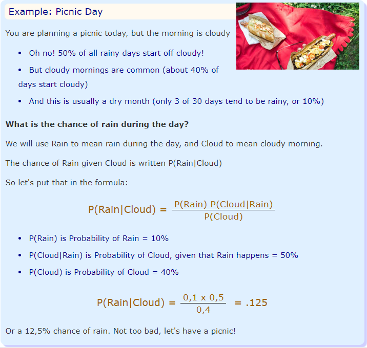
P(A|B) = ( P(A)*P(B|A) ) / P(B)

Which tells us: how often A happens given that B happens, written P(A|B) When we know: how often B happens given that A happens, written P(B|A) and how likely A is on its own, written P(A) and how likely B is on its own, written P(B)

Example application of Bayes Theorem to predict rain [1]

Difference between P(A|B) and P(A,B)

Suppose we are throwing 2 6-sided dice and suppose that condition ‘A’ is the the numbers of the top faces of the two dice sum up to 7, and condition ‘B’ is that die number 2 shows 1.

What is P(A,B)? There is only 1 way in which this can happen and it is die 2 must show a 1, and the other a 6. As there are 36 possibilities that we all assume to have equal probability, P(A,B) = 1/36.

What is P(A|B)? We know that die 2 is a 1. So the only way for the sum to be 7 is for die 1 to be a 6. As there are 6 possibilities for die 1, P(A|B) = 1/6 [2]

Naive Bayes’ Theorem

The term naive is used for real because there is a naive assumption is this theorem, which usually is not correct in real world, but makes the computation very easy. Therefore, it is highly used while solving real world problems. The naive assumption is all the events are independent of each other.

Therefore Naïve Bayes Classifier makes two simplifying assumptions

Bag of Words Assumption Assume word position doesn’t matter
Conditional Independence (Naïve Bayes) Assumption Assume the feature probabilities 𝑃(𝑓𝑖|𝑐) are independent given the class 𝑐

Probabilistic Language Modeling

Goal: to assign a probability to a sequence of words (phrase, sentence, text)

Noisy Channel Example: MT

Given an observed sequence of English words, presumably generated by translating from Turkish, what is the most likely source Turkish sentence, that could have given rise to this translation?

p(x y) models the translation process

Machine Translation
- P(high winds today) > P(large winds today)
Spelling Correction
- The office is about ten minuets from my house
- P(about ten minutes from) > P(about ten minuets from)
Speech Recognition
- P(I saw a van) » P(eyes awe of an)
Summarization, question-answering

Markov Assumption:

The probability of a word depends only on the previous word.

Markov Models:

The class of probabilistic models that assume we can predict the probability of some future unit without looking too far into the past.

N-gram

N-gram: The simplest model that assigns probabilities to sentences and sequences of words
Unigram: Also known as bag of words model
P(jumps the quick brown fox) ~ P(jumps)
Bigram (2-gram): Condition on the previous word
P(jumps the quick brown fox) ~ P(jumps fox)
Unigram (3-gram):
P(jumps the quick brown fox) ~ P(jumps brown fox)
N-gram: uses N-1 words into the past

Estimating N-gram Probabilities

The Maximum Likelihood Estimate (MLE)
estimates for the parameters of an N-gram model by getting counts from a corpus, and normalizing the counts so that they lie between 0 and 1

𝑃(𝑤𝑖	𝑤𝑖−1) = 𝐶𝑜𝑢𝑛𝑡(𝑤𝑖−1 𝑤𝑖) / 𝐶𝑜𝑢𝑛𝑡(𝑤𝑖−1)

P(food | to) = 0

Such a phrase did not occur in the corpus.
Grammatical disallowing???
… related to food …
… right to food …
Data sparsity

Extrinsic evaluation of LMs

Evaluating the performance of a LM by embedding it in an application and measuring how much the application improves spelling corrector, speech recognizer, MT system

Intrinsic evaluation of LMs

Evaluates the performance of a LM independent of any application.

Training Set: Dataset used to train parameters of our model. Test Set: An unseen dataset that is different from our training set, used to test our model Development (Held-out) Set: An additional training corpus to set the metaparameters

Perplexity (PP)

Perplexity is the inverse probability of the test set, normalized by the number of words

𝑃𝑃(𝑤1 𝑤2 𝑤3 … 𝑤𝑁) = 𝑃(𝑤1 𝑤2 𝑤3 … 𝑤𝑁) (-1/N)

Solution to Data Sparsity

Smoothing

Any corpus is limited.

Perfectly acceptable word sequences is missing
They should not receive 0 probability
Data sparsity cause two problems:
Underestimating the probability of all sort of words that might ocur
One 0 will cause the whole probability to become 0
Perplexity (inverse probability) cannot be calculated (can’t divide by 0)

Smoothing

Steal a bit of probability mass from some more frequent events and give it to the events we’ve never seen before

Smoothing types

Simple Smoothing Algorithms
- add-1 (Laplace) smoothing: Pretend each word occured one more time than it did. Just add one to all the counts!
- add-k smoothing: Add a fractional count 𝑘 (like 0.05, 0.01 How are we going to choose 𝑘 ? We will optimize it over the dev dataset.
Advanced Smoothing Algorithms
- Backoff and interpolation: If we don’t have enough context to estimate a probability, it helps to use less context
  - Backoff
    - Use trigram if you have enough evidence
    - otw bigram
    - otw unigram
  - Interpolation
    - Mix trigram, bigram and unigram
- Good-Turing smoothing: Use the count of things we’ve seen once to help estimate the count of things we’ve never seen
  - Nc = Frequency of frequency c
  - Nc = the count of things we’ve seen c times
  - Let’s use our estimate of things-we-saw-once to estimate the new things.
  - 3/18 (because N1=3) 𝑃∗(𝑢𝑛𝑠𝑒𝑒𝑛) = 𝑁1/𝑁
  - 𝑐∗ = (𝑐 + 1)𝑁𝑐+1/𝑁𝑐
- Kneser-Ney smoothing
  - Evolved from absolute-discounting interpolation, which makes use of both higher-order (i.e., higher-n) and lower-order language models, reallocating some probability mass from 4-grams or 3-grams to simpler unigram models.
  - C𝑜𝑢𝑛𝑡(●𝑤)
  - Number of unique context in which w appears
  - Number of words which precedes w
  - C𝑜𝑢𝑛𝑡(●●)
  - Number of bigram types

11. Text Classification

Sentiment Analysis: Positive or negative

Classification Approaches

Rule-based Approaches: Rules based on combinations of words or other features
- Accuracy can be high, But building and maintaining these rules is expensive
Supervised Machine Learning: Naïve Bayes Classifier
- Bag-of-words representation
  - The positions of words in a text are ignored
  - Only the frequency of words are used

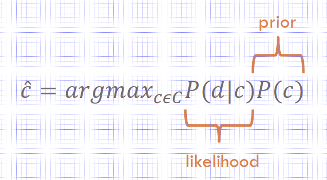
Prior: How often does this class occurs?
- We can just count the relative frequencies in a corpus
𝑃(𝑐) = 𝑁𝑐 / 𝑁𝑑𝑜𝑐𝑠
𝑁𝑐: Total number of documents labeled with class 𝑐
Ndocs: Total number of documents
Likelihood: A document can be represented as a set of features
    maximum posterior probability (MAP) ~ most likely class

Evaluating Multi-Class Classification Task

Multi-Class Classification Task

Two types of Multi-Class Classification Tasks

Any-of or multi-label classification: An item can belong to 0, 1, or >1 classes
One-of or multinomial classification: Classes are mutually exclusive, each item belongs to exactly one class

If we have more than one class, how do we combine multiple performance measures into one quantity?

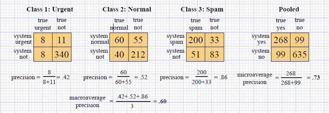
Macroaveraging: Compute performance for each class, then average.
Microaveraging: Collect decisions for all classes, compute contingency table, evaluate.

Recall: Fraction of docs in class i classified correctly. Precision: Fraction of docs assigned class i that are actually about class i.

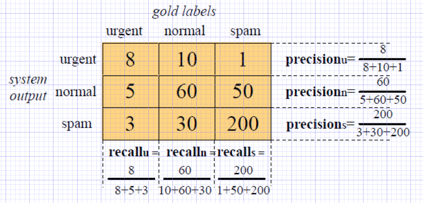
Microaverage is dominated by the more frequent class
Macroaverage is a better choice when performance on all classes is equally important

12 Sentiment Analysis

The Scherer typology of affective states

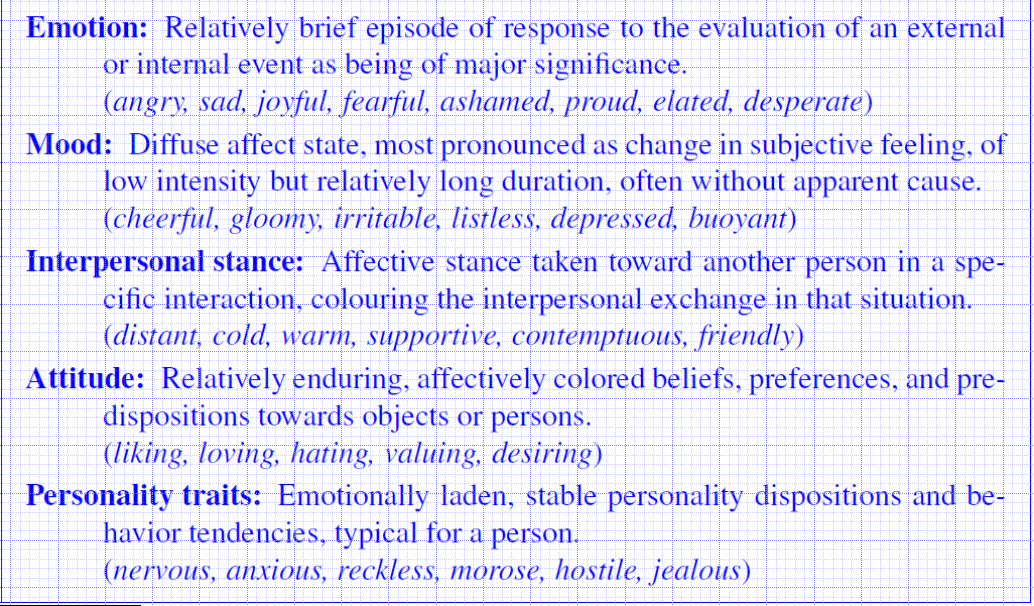
Sentiment analysis is the detection of attitudes

Holder (source) of attitude
Target (aspect) of attitude
Type of attitude
- From a set of types
  - Like, love, hate, value, desire, etc.
- Or (more commonly) simple weighted polarity:
  - positive, negative, neutral, together with strength
Text containing the attitude
- Sentence or entire document
Simplest task: Opinion extraction-Opinion mining-Sentiment mining-Subjectivity analysis
- Is the attitude of this text positive or negative?
- Linguistic or lexicon-based: Easier
  - Simple case: Taking the average of Word polarities
  - Requires domain-specific lexicons
    - Small
      - Negative for room size in hotels reviews
      - Positive for batery size in cellphone reviews
- Supervised learning based:
  - Classification task
    - Binary (+, -) or ternary (+, -, 0)
  - Regression Task
    - Rating from 1 to 5

Baseline Algorithm

Tokenization: Deal with HTML and XML markup, Twitter mark-up (names, hash tags), Capitalization (preserve for words in all caps), Phone numbers, dates, Emoticons
Feature Extraction: Which words to use? All tokens?, Only adjectives?, How to handle negation?
Classification using different classifiers
- Naïve Bayes
- MaxEnt
- SVM
More complex:
- Rank the attitude of this text from 1 to 5
Advanced:
- Detect the target, source, or complex attitude types

Sentiment Lexicons

How to build sentiment lexicons?

Manually
- Crowd-Sourcing
Semi-Supervised Learning: use seeds
- Relies on patterns of conjunction
  - Adjectives conjoined by and have same polarity
    - Fair and legitimate, corrupt and brutal
  - Adjectives conjoined by but do not
    - fair but brutal
- Hatzivassiloglou and McKeown
  - Step 1: Create seed lexicon
  - Step 2: Find cues to candidate similar words
  - Step 3: Build a polarity graph
  - Step 4: Clustering the graph
- Turney Algorithm
  - Words with similar polarity tend to occur nearby each other
  - Step 1: Extract two-word phrases
  - Step 2: Learn polarity of each phrase
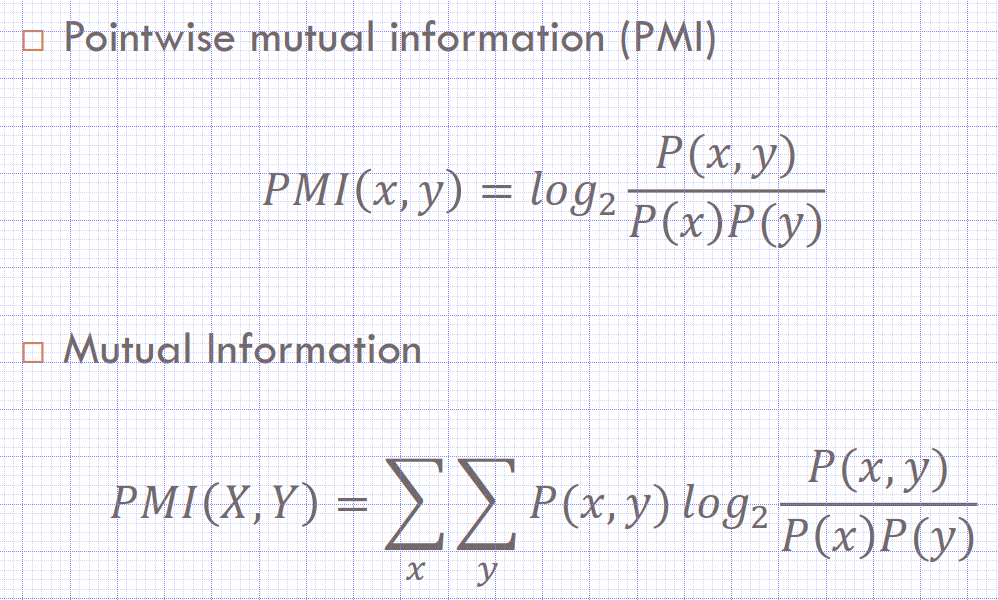
    - Mutual Information (MI): The mutual information of two random variables is a measure of the mutual dependence between the two variables. It quantifies the “amount of information” obtained about one random variable, through the other random variable. MI refers to the average of all possible events. Pointwise mutual information (PMI) refers to single events
  - Step 3: Rate a review by the average polarity of its phrases
  𝑃𝑀𝐼(𝑥, 𝑦) = 𝑙𝑜𝑔2 (𝑃(𝑥, 𝑦) / (𝑃(𝑥)𝑃(𝑦))

𝑃(𝑤) = 𝐶𝑜𝑢𝑛𝑡(𝑤) / 𝑁   𝑃(𝑤1, 𝑤2) = 𝐶𝑜𝑢𝑛𝑡(𝑤1,𝑤2) / 𝑁

    * Relies on neighborhood co−occurrence
    𝑃𝑜𝑙𝑎𝑟𝑖𝑡𝑦 (𝑝ℎ𝑟𝑎𝑠𝑒) = 𝑃𝑀𝐼 (𝑝ℎ𝑟𝑎𝑠𝑒, "𝑒𝑥𝑐𝑒𝑙𝑙𝑒𝑛𝑡") − 𝑃𝑀𝐼 (𝑝ℎ𝑟𝑎𝑠𝑒, "𝑝𝑜𝑜𝑟")

* Using WordNet
    * Step 1: Create positive and negative seed word lexicon.
    * Step 2: Extend the lexicon with synonyms and antonyms
    * Step 3: Repeat, following chains of synonyms
    * Step 4: Filter

Summary of Semi-Supervised Learning of Sentiment Lexicons

Intuition
- Start with a seed set of words (‘excellent’, ‘awful’)
    - Try to choose seed words that are
        - domain-independent
        - not commonly used in negated form
            - The movie was not very good. (common)
            - The movie was not excellent. (not common)
    -Find other words that have similar polarity:
        - Using “and” and “but”
        - Using words that occur nearby in the same document
        - Using WordNet synonyms and antonyms

Advantages:
    - Can be domain-specific
    - Can be more robust (more words)

Supervised Learning
- Enormous number of on-line reviews available
- Each review has
  - the text of the review and
  - an associated review score
    - from 1 star to 5 stars
    - scoring 1 to 10
- This review score can be used as supervision:
  - positive words: more likely to appear in 5-star reviews
  - negative words: more likely to appear in 1-star reviews
- Potts’s Algorithm
  - How likely is each word to appear in each sentiment class? But can’t use raw counts Instead, likelihood:

Challenges in Turkish Sentiment Analysis

Morphological Structure
- The agglutinative morphology makes it infeasible to build a (polarity) lexicon that would contain all variants of Turkish words
Complexity of negation
- In Turkish there are several ways a word may be negated

13 Logistic Regression

𝑐^ is indirectly estimated from the likelihood 𝑃(𝑑|𝑐) and the prior 𝑃(𝑐)

Because of this indirection, NB is a generative model
A model that is trained to generate the data 𝑑 from the class 𝑐
We are given the class 𝑐 and are trying to predict which features we expect to see in the input 𝑑.
Discriminative model
discriminating among the different possible values of the class 𝑐

Generative vs. Discriminative Models

generative models

Language models and Naive Bayes: These are also known as joint models

conditional or discriminative models in NLP, Speech, IR (and ML generally)

We have some data of paired observations 𝑑 and hidden classes 𝑐.

Joint (generative) models: 𝑃(𝑐, 𝑑)
- Place probabilities over both observed data and the hidden stuff
- Generate the observed data from hidden stuff
- All the classic StatNLP models:
  - n-gram models, Naive Bayes classifiers, HMMs, IBM machine translation alignment models
Discriminative (conditional) models: 𝑃(𝑐 𝑑)
- Take the data as given, and put a probability over hidden structure given the data
  - Logistic regression, conditional loglinear or maximum entropy models, conditional random fields
  - Also, SVMs, (averaged) perceptron, etc. are discriminative classifiers (but not directly probabilistic)
Even with exactly the same features, changing from joint to conditional estimation increases performance
Conditional models can easily memorize the training set.
They are very prone to overfitting

Logistic regression

classifying into into one of two classes

Multinomial logistic regression

classifying into more than two classes
sometimes referred to within NLP as maximum entropy modeling (MaxEnt)

NB treated Hong Kong as two independent words that have nothing to do with each other. And so it counts the evidence seperately.

Naive Bayes vs. Logistic Regression

The overly strong conditional independence assumptions of Naive Bayes mean that if two features are in fact correlated naive Bayes will multiply them both in as if they were independent, overestimating the evidence.
Logistic regression is much more robust to correlated features
if two features f1 and f2 are perfectly correlated, regression will simply assign half the weight to w1 and half to w2
When there are many correlated features, logistic regression will assign a more accurate probability than Naive Bayes.
Despite the less accurate probabilities, Naive Bayes still often makes the correct classification decision.
Naive Bayes is faster to train less likely to overfit
Naive bayes, independence assumption makes stronger the hong kong in asia example, it is not in the logistic regression, if there is dependency log regression is better choice

Maximum (Conditional) Likelihood Models

Convex optimization task

Gradient descent/ascent
- Gradient: slope

14 - 1 Expectation Maximization(EM)

Incomplete data is a common problem
The EM algorithm enables parameter estimation in probabilistic models with incomplete data

14 Hidden Markov Model

Sequence Models

A sequence model (classifier)

A model whose job is to assign a label or class to each unit in a sequence
Thus mapping a sequence of observations to a sequence of labels

An HMM is a probabilistic sequence model It computes a probability distribution over possible sequences of labels And chooses the best label sequence

Markov Chain: A weighted finite automaton:

set of states Q

𝑄 = 𝑞1, 𝑞2, … , 𝑞𝑁 𝑞0, 𝑞𝐹: Start and final (acceptance) state

Transition probability matrix 𝐴

𝐴 = 𝑎01, 𝑎02, … , 𝑎0𝑁, … 𝑎𝑁𝑁

𝑎𝑖𝑗: Probability of moving from state 𝑖 to 𝑗

Markov Assumption

An observation only depends on previous m observations

1st order Markov Model: 𝑃(𝑞𝑖 𝑞1 … 𝑞𝑖−1 = 𝑃(𝑞𝑖 𝑞𝑖−1)

2nd order Markov Model

𝑃(𝑞𝑖 𝑞1 … 𝑞𝑖−1 = 𝑃(𝑞𝑖 𝑞𝑖−1𝑞𝑖−2)

The Jason Eisner task

You are a climatologist in 2799 studying the history of global warming You can’t find records of the weather in Baltimore for summer 2006 But you do find Jason Eisner’s diary Which records how many ice creams he ate each day. Can we use this to figure out the weather?

A set of hidden states: 𝑄 = 𝑞1, 𝑞2, … , 𝑞𝑁

Transitions between states: Transition probability matrix 𝐴 = 𝑎12, 𝑎13, … , 𝑎1𝑁, … 𝑎𝑁𝑁 where σ𝑗=1 𝑁 𝑎𝑖𝑗 = 1 ∀𝑖

Observations: 𝑂 = 𝑜1, 𝑜2, … , 𝑜𝑁

Observation Likelihoods (Emission Probabilities)

The probability to generate observation 𝑜𝑡 from hidden state 𝑞𝑖 𝐵 = 𝑏𝑖(𝑜𝑡)

Initial probability distribution 𝜋 = 𝜋1, 𝜋2, … , 𝜋𝑁

Given a sequence of observations O, Figure out correct hidden sequence Q of weather states (H or C) which caused Jason to eat the ice cream

Three Fundamental Problems

1) Given a specific HMM, determine likelihood of observation sequence. 2) Given an observation sequence and an HMM, discover the best (most probable) hidden state sequence 3) Given only an observation sequence, learn the HMM parameters (A, B matrix)

Likelihood: Given an HMM M = (𝐴, 𝐵) , determine the likelihood of observing sequence O. P (O M) = ?
Decoding: Given an observation sequence O and an HMM M = (𝐴, 𝐵) , discover the best (most probable) hidden state sequence Q?
Learning: Given an observation sequence O and the set of states in the HMM, learn the HMM parameters 𝐴 and 𝐵.

Likelihood Computation

The Forward Algorithm

dynamic programming algorithm Uses a table to store intermediate values O(N^2 T)

By implicitly folding each of these paths into a single forward trellis.

Part of Speech Tagging

Word Classes

Closed Class

It cannot be extended

prepositions: on, under, over, near, by, at, from, to, with
determiners: a, an, the
pronouns: she, who, I, others
conjunctions: and, but, or, as, if, when
auxiliary verbs: can, may, should, are
particles: up, down, on, off, in, out, at, by
numerals: one, two, three, first, second, third

Ambiguity is the problem

Parsing Approaches

Sources of Information

What are the main sources of information for POS tagging? Knowledge of word probabilities  man is rarely used as a verb….

Share on

Twitter Facebook Google+ LinkedIn

M. Oguz Ozcan